Handout #1

The Theory of Labor Supply - A Rudimentary Outline
 

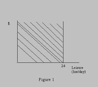
I. The Choice Set (all conceivable work/leisure - dollar combinations)

Note: the choice set is illustrated above on a daily basis, but such a representation need not be the case. The model works equally well for hours per week, weeks per year, or any other measure of time in the labor force.
 

II. The Preference Set
 

Generally, more leisure and money are preferred to less of both. Thus people would prefer to move as close as possible to the north-east region of figure 1. Theory does not have ambiguous conclusions about the trade-offs between leisure and money. Hence indifference curves illustrating individual preferences with respect to trade-offs are necessary. Theory tells us that higher indifference curves are preferred to lower ones.

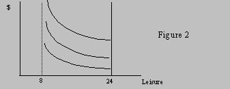
Note that having no indifference curves in the 0-8 hour leisure regions implies a preference for "sleep". No wage would induce people to give up more than 16 hours of leisure in figure 2. The exact location of the indifference curves depends on individual physical needs as well as tastes.
 

III. Constraints on Choices
 

Not all choices are available to all individuals all the time. Limitations on available work/leisure - dollar choices may exist for many reasons. Cyclical economic conditions, discrimination, limitations of individual ability are a few examples. We shall study several kinds of constraints that limit the choice set.
 

a - Arbitrary constraints (the hours of arbitrary work/leisure - dollar combinations available to the

individual)

Figure 3
 
 
 
 
 
 
 
 
 
 
 

b - Earnings capacity constraints (one can work as much as one wants at given wage rates).

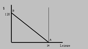
Figure 4
 
 
 
 
 
 
 
 
 

1. Question: What is the slope of the constraint AB? What is the individual's hourly wage rate represented by AB?
 

c - Variable wage constraints (when wages vary depending on hours worked).
 

1 - Overtime pay
 
 
 
 
 
 

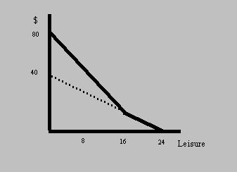
Figure 5
 
 
 
 
 
 
 
 
 
 
 
 
 
 
 

Questions:

1. After how many hours does overtime pay begin?
 

2. What are the normal and overtime rates of pay?
 

2 - progressive and regressive taxes on wages
 

Figure 6
 
 
 

Figure 7
 
 
 
 
 
 
 
 
 
 
 
 
 
 
 
 
 
 
 
 
 

Question:

3. Which figure represents the progressive and which the regressive tax?
 

3 - The Effect of Unearned Income on the Wage Constraint (free transfer payments)

A - Husband's Income on Wife's Constraint (or vice virsa)

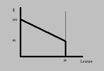
Figure 8
 
 
 
 
 
 
 
 
 
 
 
 
 

Question:

4. Assume the husband works 8 hours per day and gives all his earnings to his wife. Determine the wife's wage rate from the above diagram depicting the wife's wage constraint.
 

B - Welfare payments.

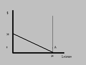
Figure 9
 
 
 
 
 
 
 
 
 
 
 
 
 
 
 
 
 

Point A represents welfare payments if individual does not work.
 

Question:

5. What is the welfare payment?
 

C. Negative Income Tax Plan

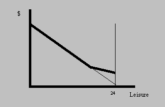
Figure 10
 
 
 
 
 
 
 
 
 
 
 
 
 
 
 

IV. Equilibrium: the Preference Set Combined with the Constraints
 

The equilibrium number of hours worked can be determined by that number of hours that maximizes the utility (or preferences) given the market constraints on the work/leisure - dollar choices. That is, the individual determines his (or her) hours of leisure and work ads that amount of hours that puts him (her) on the highest indifference curve.

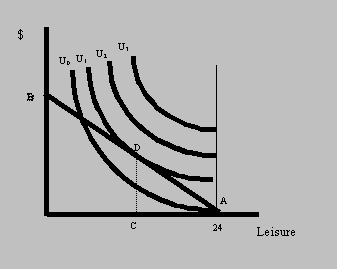
Figure 11
 
 
 
 
 
 
 
 
 
 
 
 
 
 
 
 
 

AB - constraint

AC - optimum hours worked

OC - optimum leisure hours
 

In economics terms, the equilibrium (D) can be described as that point such that
 

That is one works up until the point that the marginal disutility of work exceeds the utility gain of extra wages. In mechanical terms, this point occurs when the slope of the earnings capacity constraint (wage rate) equals the slope of the indifference curve.
 

V. Changes in Constraints
 

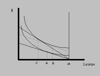
Figure 12
 
 
 
 
 
 
 
 
 
 
 
 
 
 
 
 
 
 
 

Original equilibrium A

New equilibrium C

Total effect AC

Income effect AB

Substitution effect BC
 

In general any change in wages evokes two responses. The substitution effect always causes individuals to work more (because leisure is more costly). The income effect may cause people to work more or less depending on the income elasticity of leisure. If leisure is a normal good people work less (and consume more leisure). If leisure is an inferior good people work more and consume less leisure.
 

Question:

6. Define (a) income elasticity (b) normal good and (c) inferior good. Figure 12 represents the case where leisure is a _______ good.
 

7. Draw the case where both effects reinforce each other.
 

Labor Supply Regressions
 

1 - Results of multiple regression of average weekly hours on hourly earnings and other variables for white and black males 18-64, 1980.
 

H = c - E + M + S + A - B - I
 

where

c = constant

H = mean hours worked by male wage and salary workers in census week, 1980

E = hourly wage and salary income

M = marital status (1=married)

S = schooling, in years

A = age

B = race (1=black)

I = other income
 
 
 

2 - Labor force participation for 1980 population over 65 years of age
 

N = c + E - I (Males)
 

N = c + E - I (Females)
 

where

N = percent in labor force (labor force participation rate)

E = earnings

I = other income
 
 
 

for females 16-65
 

N = c +E - I + S - K
 
 
 

where

U = unemployment rate

K = number of kids
 

Questions:

1. Do more educated women have a higher or lower labor force participation?

2. What is the effect of children on women's labor force participation?

3. Do married women work greater amounts than non-married men?

4. Is the male labor supply curve for hours "backward bending"?